
Be aware to the reader: That is the eleventh in a sequence of articles I am publishing right here taken from my guide, “Investing with the Development.” Hopefully, you’ll find this content material helpful. Market myths are usually perpetuated by repetition, deceptive symbolic connections, and the entire ignorance of information. The world of finance is stuffed with such tendencies, and right here, you may see some examples. Please remember that not all of those examples are completely deceptive — they’re typically legitimate — however have too many holes in them to be worthwhile as funding ideas. And never all are immediately associated to investing and finance. Take pleasure in! – Greg
Market Valuations
As a result of secular markets are outlined by long-term swings in valuations, let us take a look at the Worth Earnings (PE) ratio and research its historical past. Robert Shiller created a helpful measure of PE valuation that makes use of trailing (precise) earnings, averaged over a 10-year interval. Here is how it’s calculated:
- Use the yearly incomes of the S&P 500 for every of the previous 10 years.
- Alter these earnings for inflation, utilizing the CPI (i.e. quote every earnings determine in present {dollars}).
- Common these values (i.e., add them up and divide by 10), giving us e10.
- Take the present Worth of the S&P 500 and divide by e10.
Determine 8.1 exhibits the S&P Composite on a month-to-month foundation adjusted for inflation, again to 1871, with a regression line so you will get a really feel (visually) of the place the present value is relative to the long-term development of costs. The decrease plot is the Shiller PE10 plot, with peaks and troughs recognized with their values. You’ll be able to see that each one prior secular bears ended with PE10 as a single digit (4.8, 5.6, 9.1, and 6.6). The PE10, on March 9, 2009, solely bought all the way down to 13.3, which is significantly greater than the extent reached by all prior secular bear lows. Based mostly on this easy analogy, I feel now we have but to see the secular bear low for this cycle. Keep in mind, it doesn’t imply that the costs must go decrease than they did in 2009; it simply means the PE10 ought to drop to single digits. Keep in mind, PE is a ratio of Worth over Earnings. To make the ratio smaller, both the value can decline, the earnings can enhance, or a mix of each.
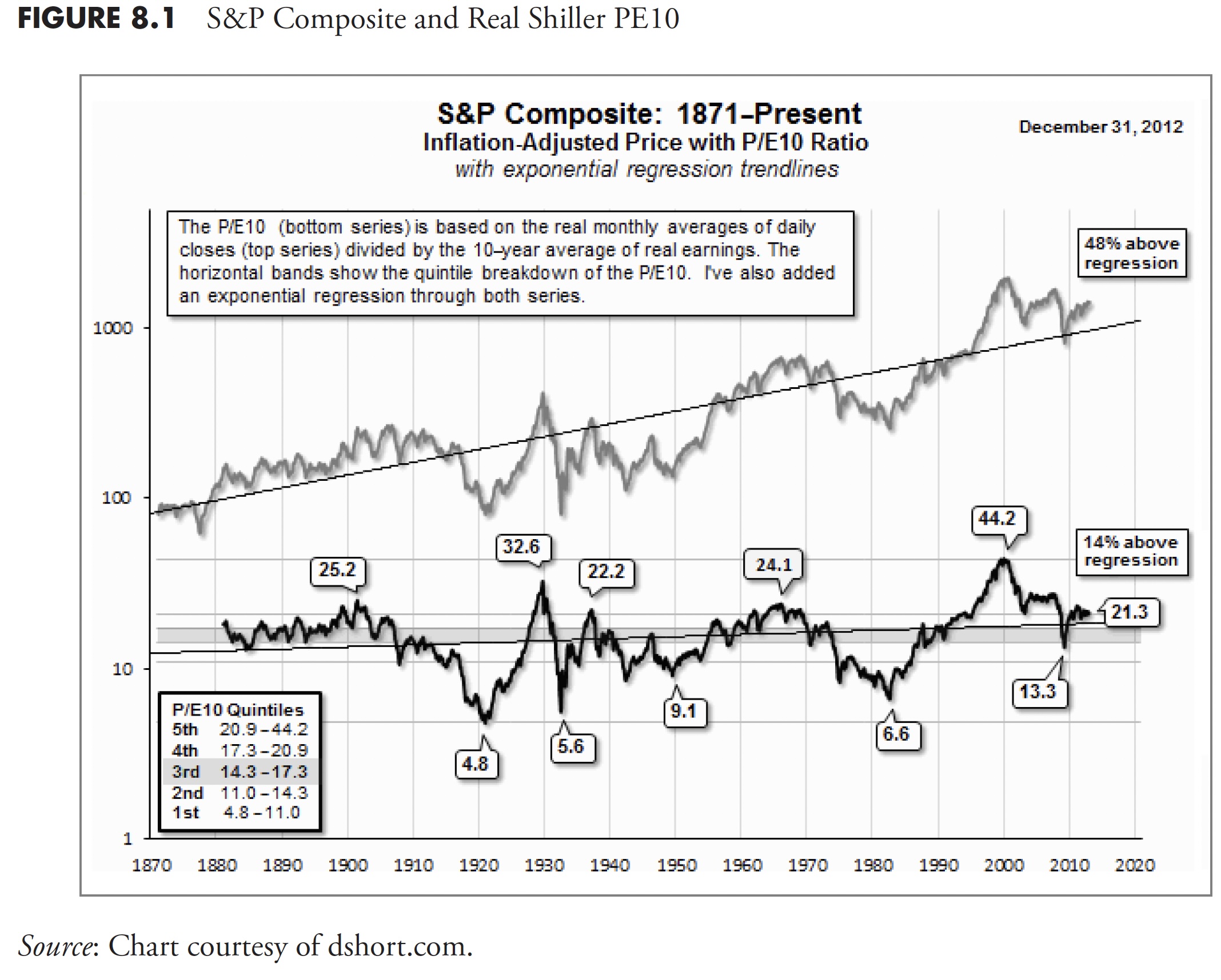
As of December 31, 2012, the PE10 is at 21.3. Referencing the small field within the decrease left nook exhibits that this worth is within the fifth quintile of all of the PE knowledge. Based mostly on this evaluation, the market is overvalued.
So when the monetary information noise is consistently parading analysts by touting the PE as overvalued or undervalued, you’ll be able to rely on the truth that they’re utilizing the ahead PE ratio. The ahead ratio is the guess of all of the earnings analysts. They’re not often appropriate. Ignore them.
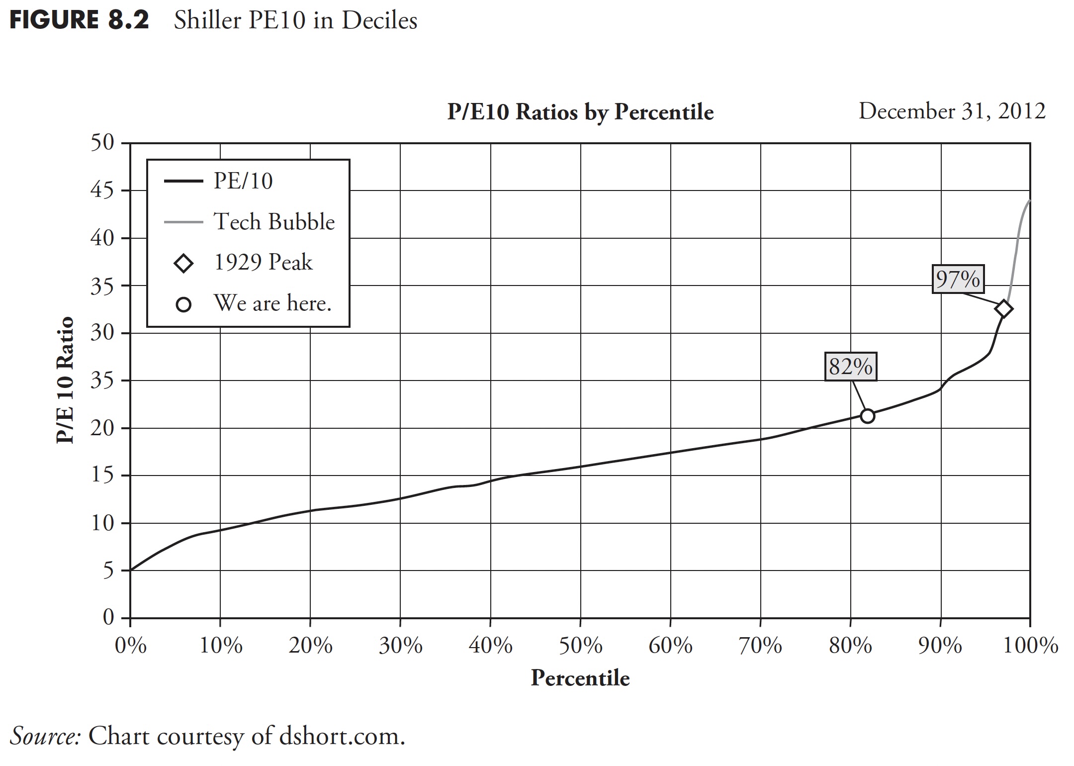
Lastly, Determine 8.2 exhibits the PE10 in 10 % increments or deciles. It exhibits the acute stage reached within the late Nineties from the tech bubble, it exhibits the 1929 peak, and it exhibits that, as of December 31, 2012, we’re on the 82nd percentile of PE10. This places the PE10 overvalued on a relative foundation, and likewise on an absolute foundation, as proven in Determine 8.1. Keep in mind, PE10 used actual reported (trailing) earnings, not ahead (guess) earnings. As Doug Brief says on his web site at dshort.com: A extra cautionary remark is that when the PE10 has fallen from the highest to the second quintile, it has ultimately declined to the primary quintile and bottomed in single digits. Based mostly on the most recent 10-year earnings common, to succeed in a PE10 within the excessive single digits would require an S&P 500 value decline beneath 540. After all, a happier various can be for company earnings to proceed their robust and extended surge. If the 2009 trough was not a PE10 backside, when would we see it happen? These secular declines have ranged in size from greater than 19 years to as few as three. As of December 31, 2012, the decline in valuations was approaching its thirteenth 12 months.
Secular Bear Valuation
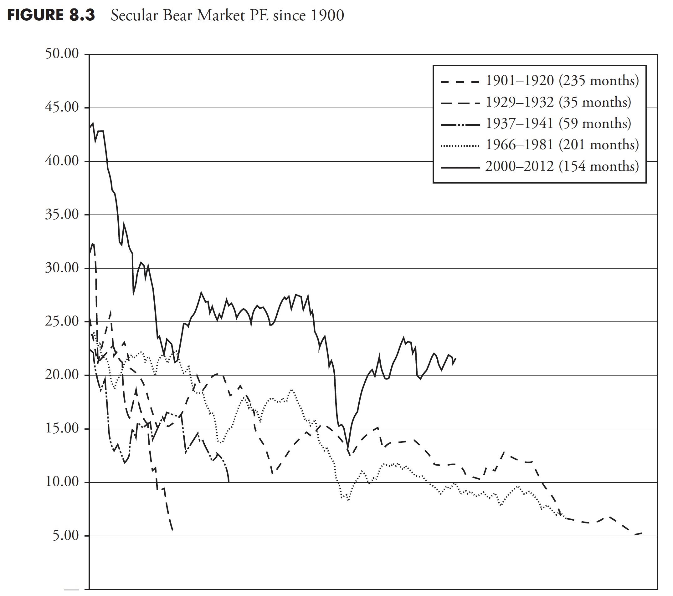
Determine 8.3 exhibits the Shiller PE10 month-to-month for all of the previous secular bear markets since 1900, with the present secular bear (as of 2013) in daring. What is de facto attention-grabbing about this chart is that many of the secular bears started with PE Ratios within the 20 to 30 vary and ended with them within the 5 to 10 vary. The present secular bear started with a PE within the mid-40s and is now solely again all the way down to the extent that the earlier secular bears started. That would suggest that the secular bear that started in 2000 could possibly be an extended one. These charts had been created utilizing month-to-month knowledge; if yearly knowledge had been used, the idea can be much more pronounced.
Secular Bear Valuation Composite
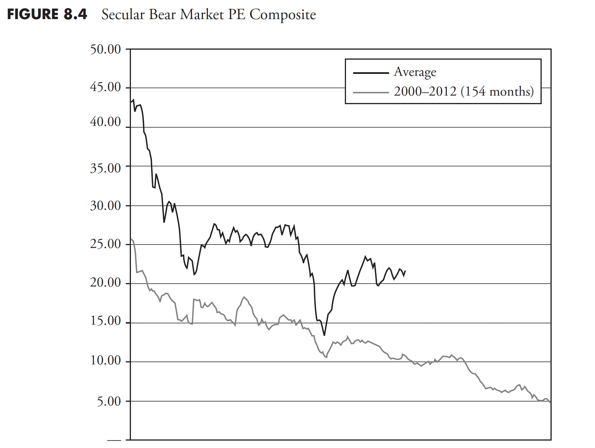
In Determine 8.4, the present secular bear market valuation is proven in daring, with the opposite line representing the common of the earlier 4 secular bears. Once more, this kind of evaluation is simply an remark and for instructional functions; you can’t make funding selections from this. Funding selections come from actionable data and evaluation.
Secular Bull Valuation
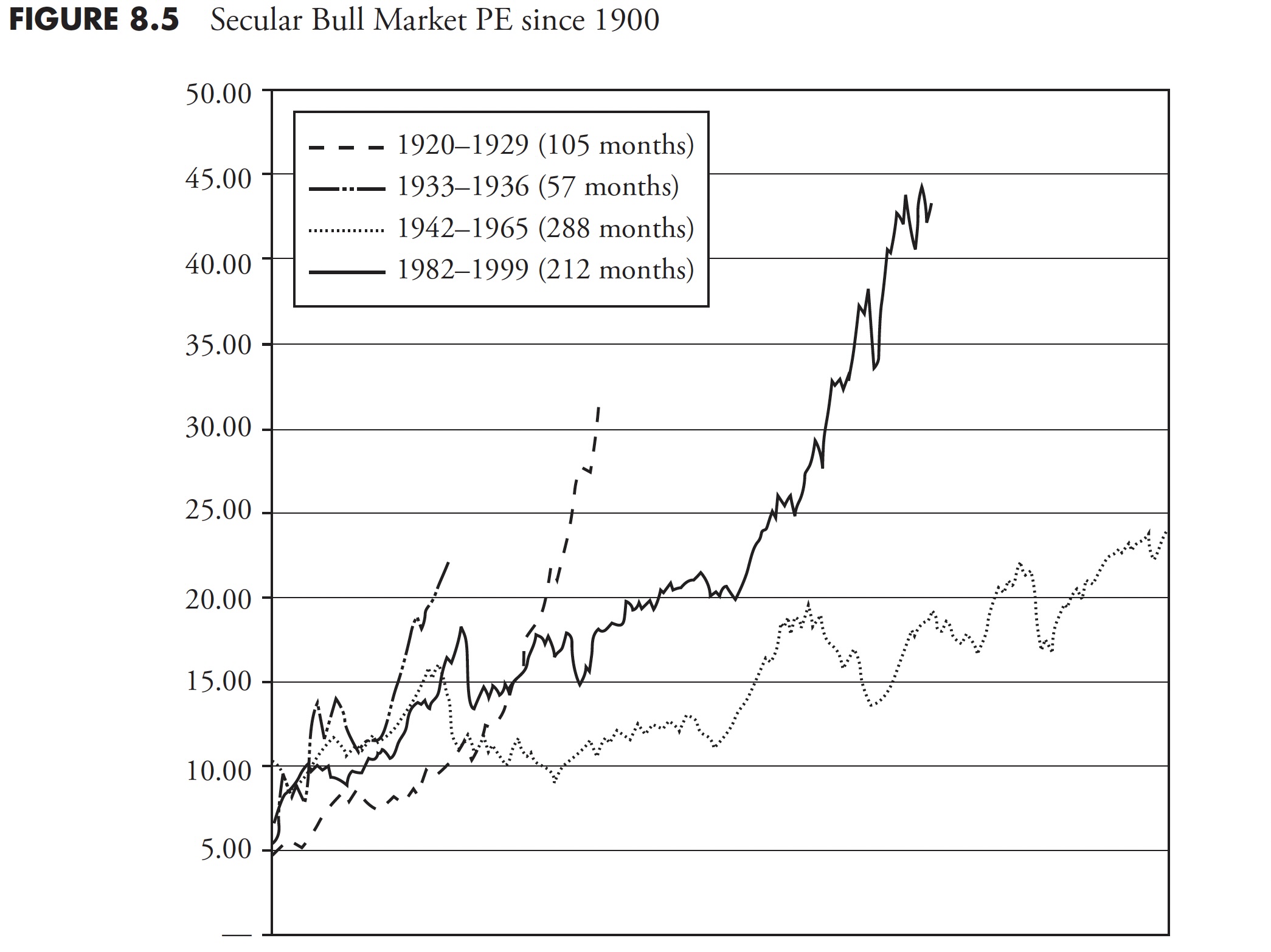
Determine 8.5 of secular bull market valuations exhibits that almost all of them start with PE ratios within the 5 to 10 (similar as the place secular bears finish) and so they finish with PE ratios within the 20 to 30 vary. The extreme secular bull of 1982 to 2000 reached unbelievable excessive valuations. I bear in mind everybody saying that this time was totally different. Unsuitable!
Secular Bull Valuation Composite
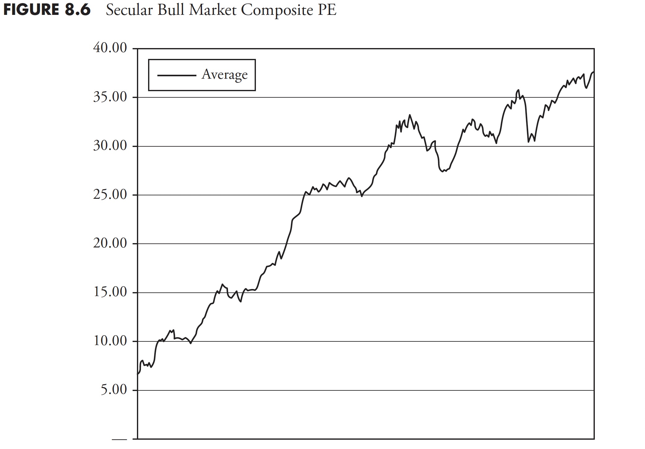
The secular bull market valuation composite is proven in Determine 8.6. It’s the common of all of the secular bull markets since 1900. Since we’re at present in a secular bear market, the common of the secular bull markets is proven by itself.
Market Sectors
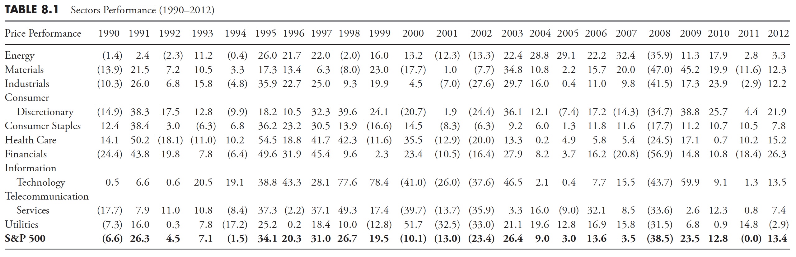
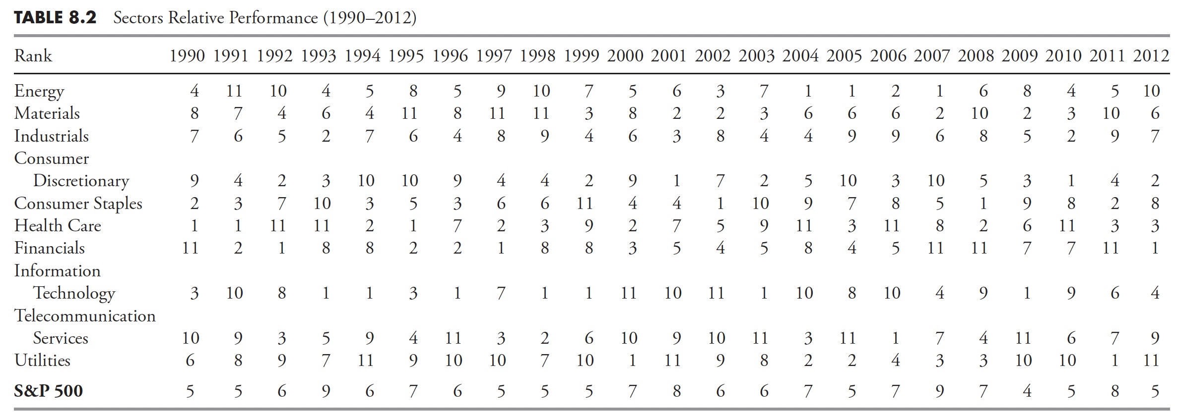
I exploit the sector definitions supplied by Customary & Poor’s, of which there are 10. The opposite major supply for sector evaluation is Dow Jones. Both is okay, I simply favor the S&P construction as a result of I’ve been utilizing it for thus lengthy. Desk 8.1 exhibits the ten sectors’ annual value efficiency since 1990, and Desk 8.2 exhibits the relative efficiency of the whole returns. When viewing a desk of relative returns as in Desk 8.2, remember that every column (12 months) is totally unbiased of the previous 12 months or following 12 months. Additionally, the relative rating exhibits that these within the high a part of the column outperformed these within the decrease a part of the column, unbiased of whether or not the returns had been optimistic, unfavourable, or a mix. One other worth of this kind of desk is to point out that choosing final 12 months’s high performer is just not a superb technique. Keep in mind, you can’t retire on relative returns.
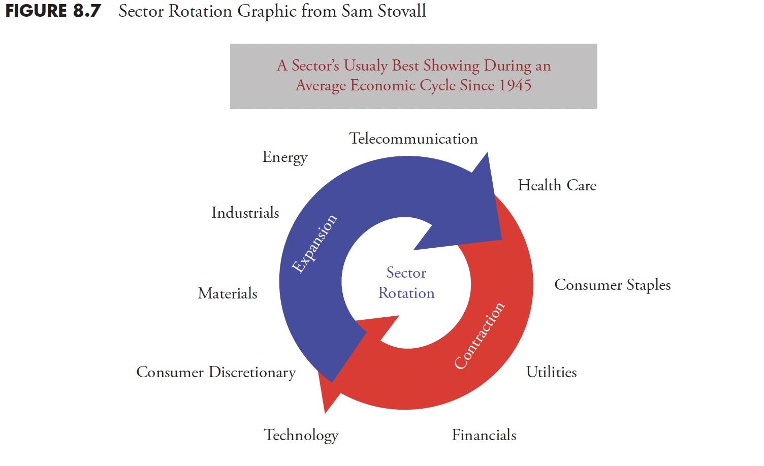
This guide doesn’t get into the assorted makes use of of sectors as investments, however the guide wouldn’t be full with out the point out of sector rotation and, particularly, how varied sectors rotate out and in of favor based mostly on the section of the enterprise cycle and the economic system. An additional delineation of sectors is their propensity to fall throughout the broad classes of offensive and defensive. Which means when the market is performing poorly, the defensive sectors will usually outperform, and when the market is performing effectively, it’s the offensive sectors which can be the highest performers.
The phases of the economic system often called financial expansions and contractions are affected by many occasions however usually boil all the way down to recessions and intervals of enlargement. It needs to be famous, nevertheless, that not all contractions find yourself being recessions. The phases can then be damaged down into early cycle, mid-cycle, and late cycle segments of the complete cycle. There’s quite a lot of literature out there to cowl all these particulars, however the level of this dialogue is to point out the rotational motion of the assorted sectors via the financial cycle.
Determine 8.7 is a graphic exhibiting the sectors and the place they fall within the cycle. It exhibits the rotation of sectors throughout a median financial cycle for the previous 67 years and is courtesy of Sam Stovall, chief fairness strategist, S&P Capital IQ. Sam wrote top-of-the-line books on sector rotation years in the past, Customary & Poor’s Sector Investing: Learn how to Purchase the Proper Inventory within the Proper Trade at The Proper Time, however is at present out of print as of 2013.
One other wonderful research I’ve seen on the cycles throughout the phases and what sectors are affected was put out by Constancy and dated August 23, 2010 (see Desk 8.3). It clearly confirmed that, from 1963 via 2010, the next sectors had been strongest throughout the varied phases. In every cycle, the top-performing sectors are proven, with the primary being the most effective of the 4 and the final being the worst of the highest 4, which continues to be the fourth finest out of the ten sectors.
It was attention-grabbing to notice on this research that in the entire three cycles, Utilities and Healthcare had been the 2 worst-performing of all 10 of the sectors (not proven). They solely ranked within the high 4 throughout precise recessions. Since recessions are often recognized by the NBER a few 12 months after they start and someday not till they’ve ended, this isn’t data that you would be able to make funding selections with.
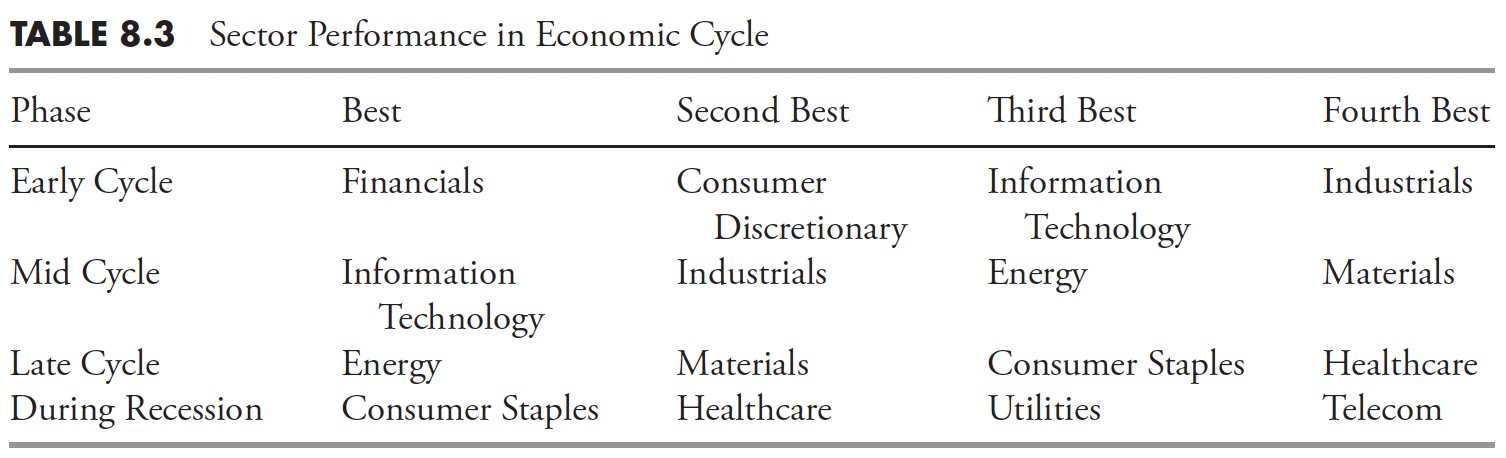
Nevertheless, you need to use a momentum evaluation and all the time be within the high 4 sectors and possibly do effectively. Clearly, that is actually higher than buy-and-hold or index investing.
Determine 8.8 exhibits the S&P 500 within the high plot and my Offensive-Defensive Measure within the decrease plot. The idea of the Offensive-Defensive Measure is straightforward.
The Offensive Elements
- Client Discretionary
- Financials
- Industrials
- Info Expertise
The Defensive Elements
- Client Staples
- Utilities
- Healthcare
- Telecom
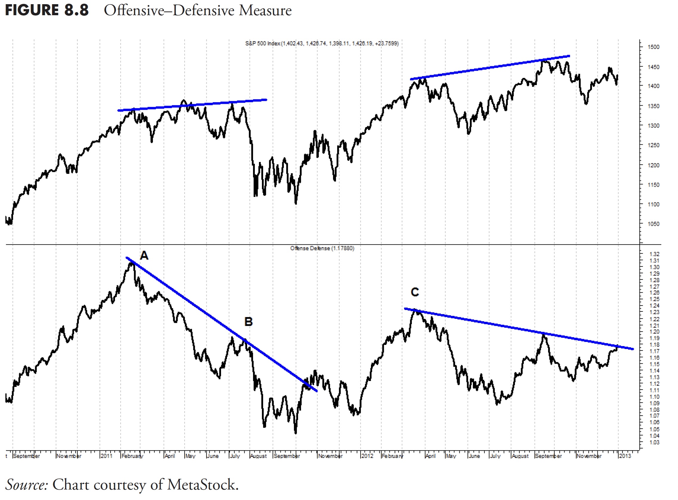
You’ll be able to see that the rally from the left facet of the chart to level A (February, 2011) was robust; nevertheless, based mostly on the change from offensive to defensive sectors that occurred at level A, the buyers had been clearly involved in regards to the market. Whereas the market traded sideways for months (see high plot), the defensive sectors had been clearly within the lead, inflicting the offense-defense measure to say no. The measure declined considerably, and it wasn’t till level B (July 2011) that the market lastly gave up and headed south.
Sector Rotation in 3D
Julius de Kempenaer has created a novel method of visualizing sector-rotation, or, extra usually, “market-rotation,” in such a method that the relative place of all components in a universe (sectors, asset lessons, particular person equities, and so forth.) may be analyzed in a single single graph as an alternative of getting to flick through all attainable mixtures. This graphical illustration known as a Relative Rotation Graph or RRG. As of 2013, Julius is now working along with Trevor Neil to additional analysis and implement using RRGs within the funding means of funding corporations, funds, and particular person buyers. Extra data may be discovered on their web site www.relativerotationgraphs.com.
A Relative Rotation Graph takes two inputs that collectively mix into an RRG. I am going to use the S&P Sectors for this dialogue. Step one is to give you a measure of relative energy of a sector versus the S&P 500; that is achieved by taking a ratio between every sector and the S&P 500. Analyzing the slope and tempo of those particular person RS strains offers a reasonably good clue about particular person comparisons versus their benchmark. These uncooked RS strains reply “good” or “unhealthy.” Nevertheless, they don’t reply “how good” or “how unhealthy” or “finest” and “worst.” The explanation for that is that Uncooked RS values (sector/benchmark) for the assorted components within the universe are like apples and oranges, as they can’t be in contrast based mostly on their numerical worth.
Taking the relative positions of all components in a universe under consideration in a uniform method permits “rating.” This course of normalizes the assorted ratios in such a method that their values may be in contrast as apples to apples, not solely towards the benchmark but additionally towards one another. The ensuing numerical worth is called the JdK RS-Ratio—the upper the worth, the higher the relative energy. Moreover, not solely the extent of the ratio, but additionally the route and the tempo at which it’s transferring, impacts the end result. An idea much like the well-known MACD indicator is used to measure the Fee of Change or Momentum of the JdK RS-Ratio line. Right here additionally, you will need to preserve comparable values so one other normalization algorithm is utilized to the ROC; this line is called the JdK RS-Momentum. The RRG now has JdK RS-Ratio for the abscissa (X axis) and the JdK RS-Momentum for the ordinate (Y axis). Graphically, the rotation appears to be like like Determine 8.9.
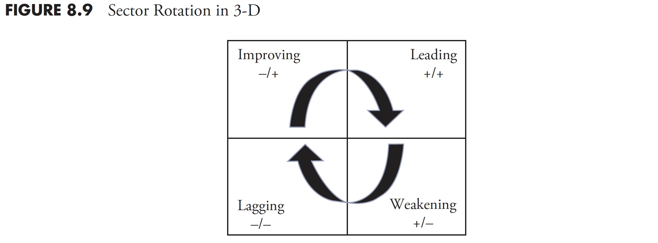
In Determine 8.10, the sectors which can be exhibiting robust relative energy, which continues to be being pushed greater by robust momentum, will present up within the top-right quadrant. By default, the Fee of Change will begin to flatten first, then start to maneuver down. When that occurs, the sector strikes into the bottom-right quadrant. Right here, we discover the sectors which can be nonetheless exhibiting optimistic relative energy, however with declining momentum. If this deterioration continues, the sector will transfer into the bottom-left quadrant. These are the sectors with unfavourable relative energy, which is being pushed farther down by unfavourable momentum. As soon as once more, by default, the JdK RS-Momentum worth will begin to transfer up first, which is able to push the sector into the top-left quadrant. This the place relative energy continues to be weak (i.e. < 100 on the JdK RS-Ratio axis) however its momentum is transferring up. Lastly, if the energy persists, the sector might be pushed into the top-right quadrant once more, finishing a full rotation.
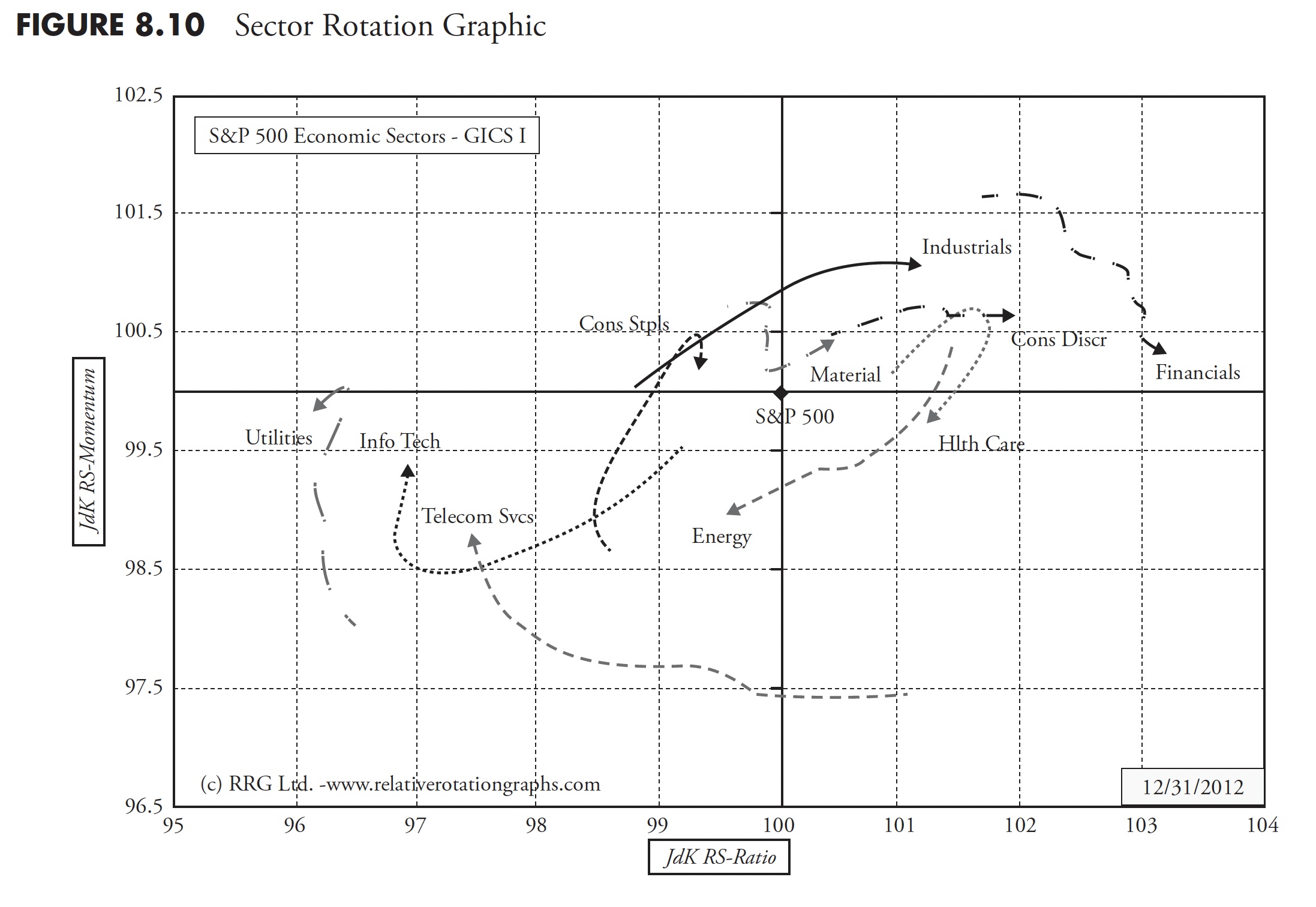
The subsequent step is so as to add the third dimension, time, to the plot to visualise the info on a periodic foundation and in reality, considerably like watching a flip chart or animation in which you’ll see the motion of every of the sectors across the chart as proven in Determine 8.10.
This know-how, in static kind, is obtainable on the Bloomberg skilled service since January 2011 as a local perform (RRG<GO>) the place customers can set their desired universes, benchmarks, lookback intervals, and so forth. On their aforementioned web site, Julius and Trevor preserve quite a lot of RRGs, static and dynamic (animated rotation), on in style universes just like the S&P 500 sectors (GICS I & II). A number of skilled in addition to retail software program distributors and web sites are working to embed the RRG know-how of their merchandise, which ought to make this distinctive visualization instrument out there to a wider viewers.
Asset Lessons
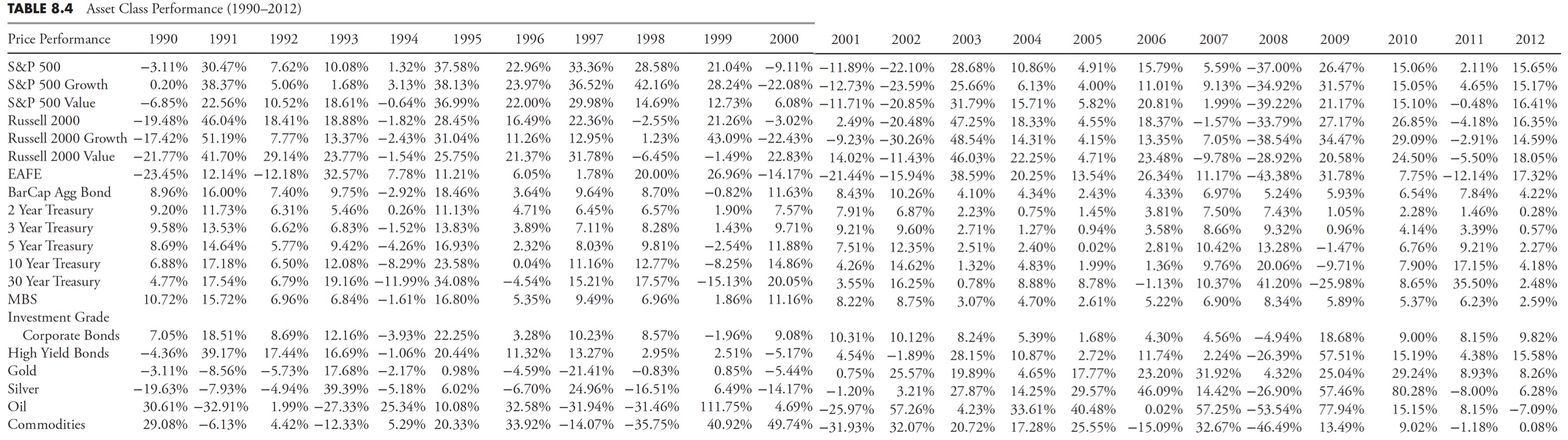
Asset lessons may be analyzed precisely the identical as market sectors. The one limitation is that they aren’t tied as intently to financial cycles as sectors, so it’s harder to establish these which can be offensive or defensive. Desk 8.4 exhibits the value efficiency of a large number of asset lessons. Keep in mind, this desk is barely exhibiting the annual efficiency of every asset for every year since 1990, whereas Desk 8.5 has the asset lessons ranked every year numerically. Usually, this kind of desk is proven with a number of colours, however considerably tough in a black-and-white guide, so rankings are proven. Once more, do not forget that the rankings solely present the relative efficiency, and every year is completely unbiased of the previous or following 12 months.

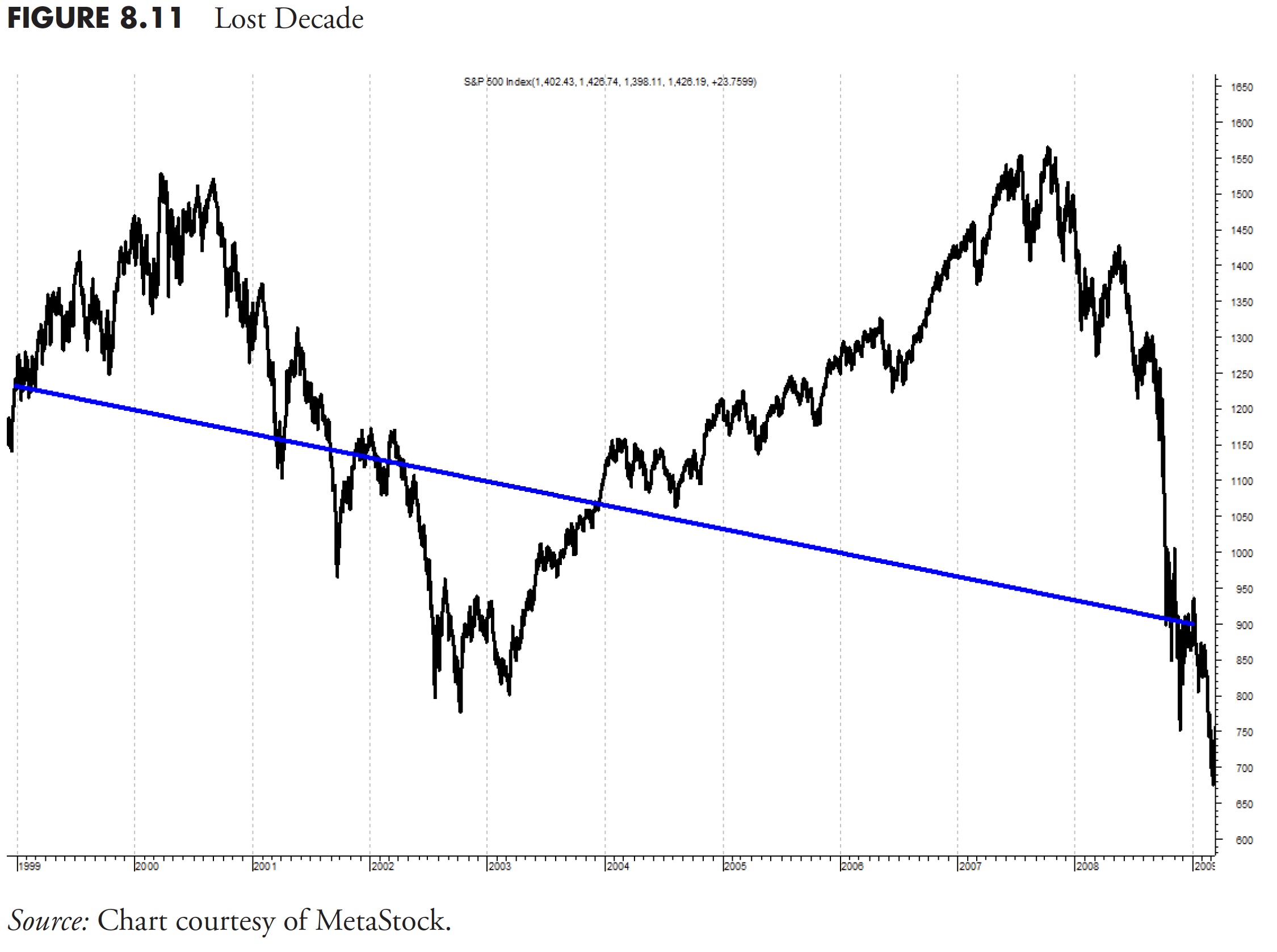
The Misplaced Decade
Determine 8.11 exhibits the S&P 500 Complete Return from December 31, 1998, to December 31, 2008. Two large bear markets and two good bull markets. If in case you have a method that might seize a superb portion of these bull markets and keep away from a superb portion of these bear markets, you’ll do very well. Purchase and maintain has misplaced cash over this era.
I get requested on a regular basis, “Are we going to have one other bear market?” I reply that I can assure you that we are going to; I simply don’t know when it is going to be. Nevertheless, we are able to flip to a different group of very vivid individuals from the third-largest economic system on the earth (as of 2013) and take a look at their market. Determine 8.12 is the Japanese Nikkei from December 31, 1985, to December 31, 2011, a time period of 26 years, over 1 / 4 of a century.
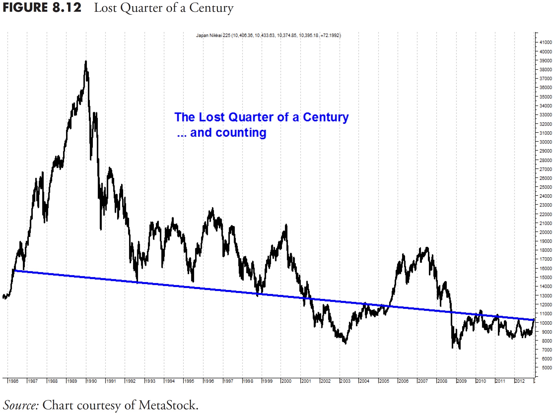
Clearly, purchase and maintain was a devastating funding technique, and the actually unhealthy information is that it nonetheless is. Determine 8.13 exhibits the up and down strikes throughout this era, during which a superb development following technique might have protected you from horrible devastation.
The proportion strikes up are proven above the plot, and the proportion strikes down are beneath the plot. These are the proportion strikes for every of the up and downs you see on the chart. There have been 5 cyclical bull strikes of better than 60 % throughout this era. There have been additionally 5 cyclical bear strikes of better than -40 %. Keep in mind, a 40 % loss requires a acquire of 66 % simply to get again to even. The small field within the decrease proper edge exhibits the decline from the market high in late December 1989 (–73.3 %). A 73 % decline requires a acquire of 285 % to get again even. Most individuals will not reside lengthy sufficient for that to occur.
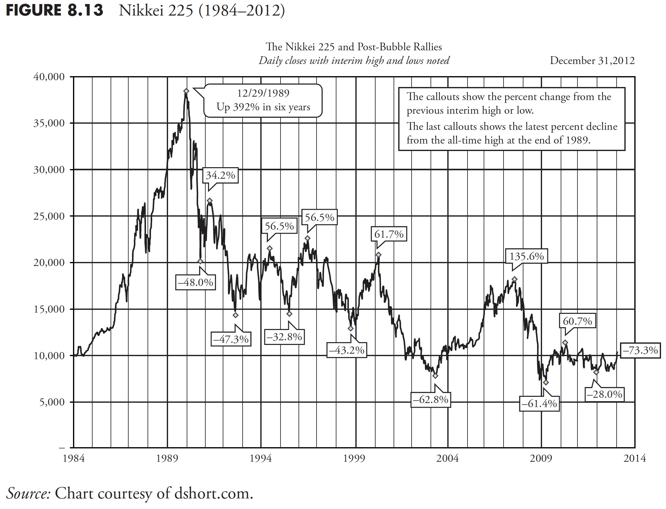
Lastly, please discover that Determine 8.13 covers roughly 30 years of knowledge and that the purpose on the precise finish (most up-to-date worth) is roughly equal to the place to begin again within the mid-Eighties; actually the misplaced three many years. Purchase and Maintain is Purchase and Hope.
Market Returns
It’s all the time good to see how the markets have carried out up to now. With the arrival of the web, globalization, minute-by-minute information, buyers have a pure tendency to deal with the brief time period. With no data of the long-term efficiency of the markets, that short-term orientation could cause one to be completely out of contact with the truth that the market doesn’t all the time go up. The next charts will present annualized returns for the S&P 500 value, whole return, and inflation-adjusted whole return over varied intervals. A majority of these charts are also referred to as rolling return charts. For example, utilizing the 10-year annualized rolling return, the info begins in 1928, so the primary knowledge level wouldn’t be till 1938 and be the 10-year annualized return from 1928 to 1938. The subsequent knowledge level can be for the 10-year interval from 1929 to 1939, the third from 1930 to 1940, and so forth.
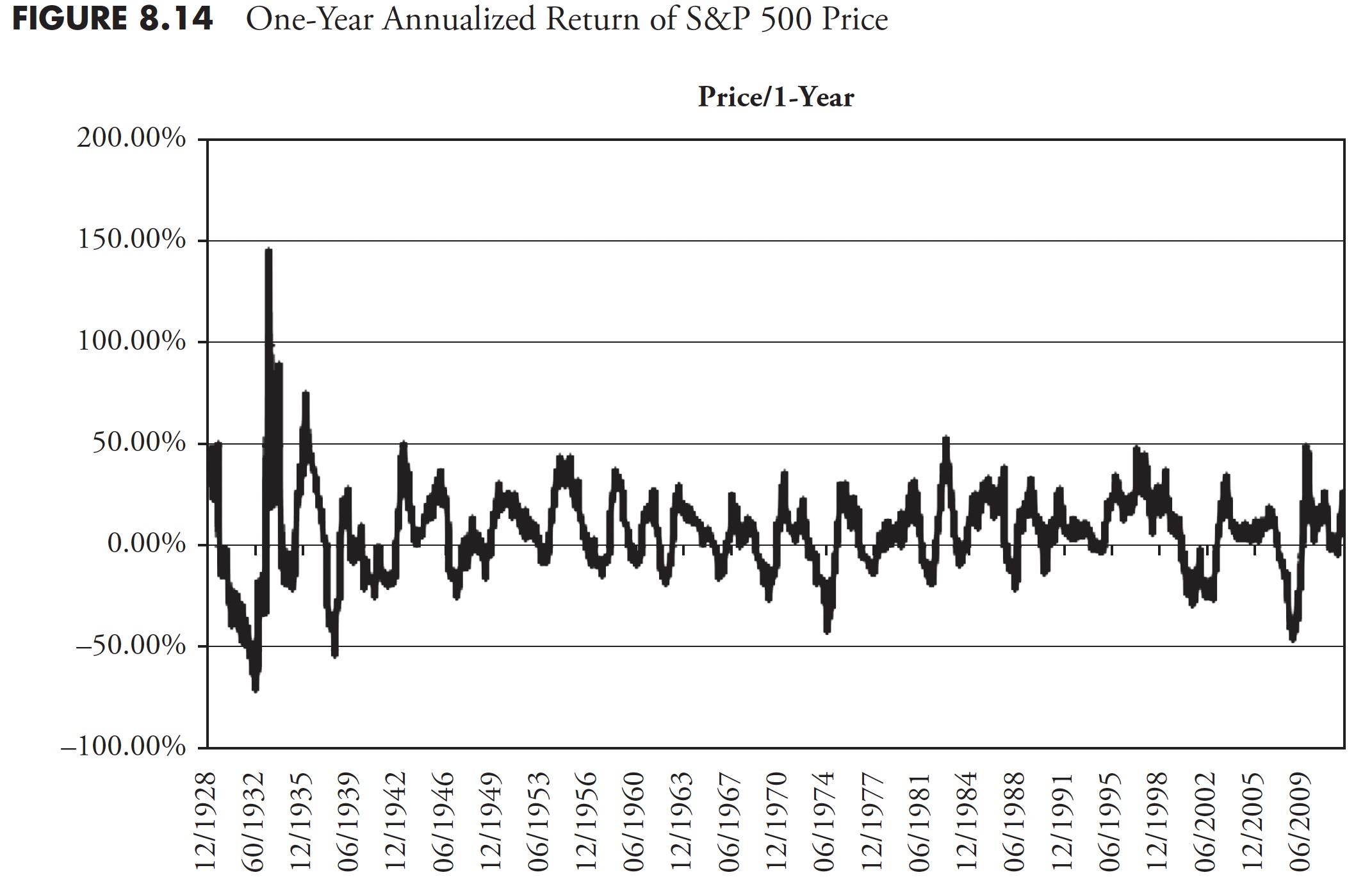
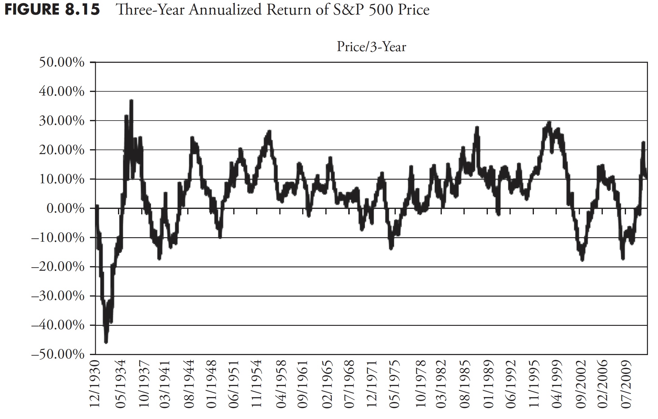
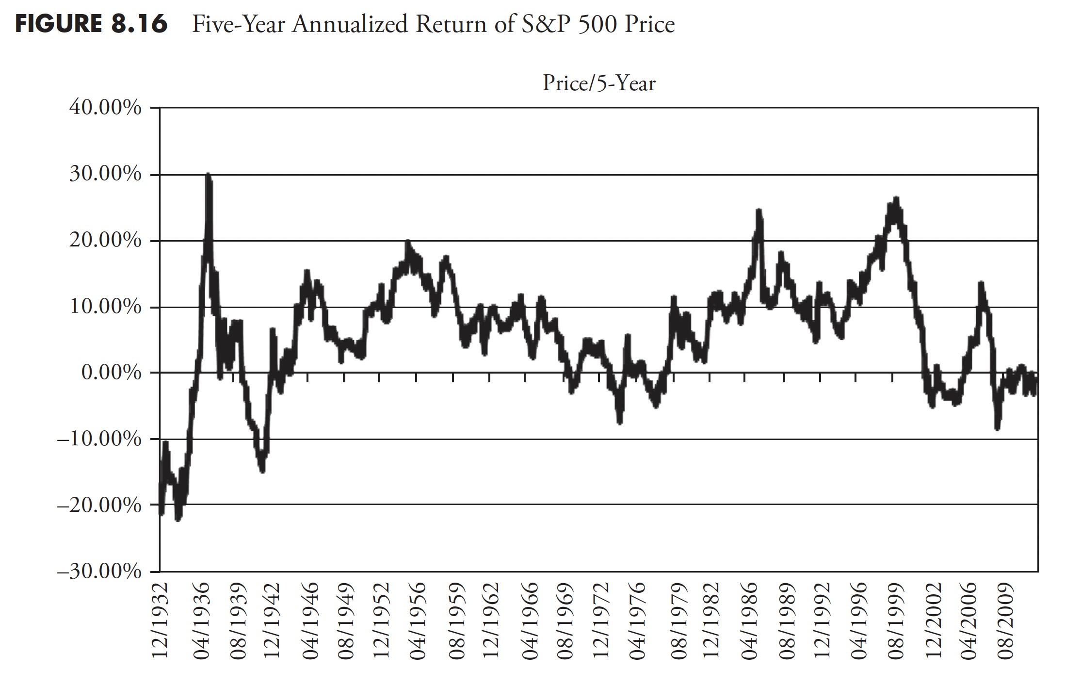
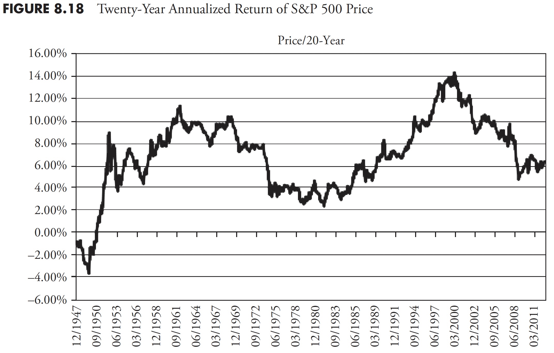
Determine 8.14 exhibits the 1-year annualized return for the S&P value. It needs to be apparent that one-year returns are all over, oscillating between highs within the 40 % to 50 % vary, and lows within the -15 % to -25 % vary. Following Determine 8.14 are the 3-year (Determine 8.15), 5-year (Determine 8.16), 10-year (Determine 8.17), and 20-year (Determine 8.18) charts of annualized returns, with the common for all the info proven within the chart caption. Following the 20-year chart is an extra evaluation for the 20-year interval.
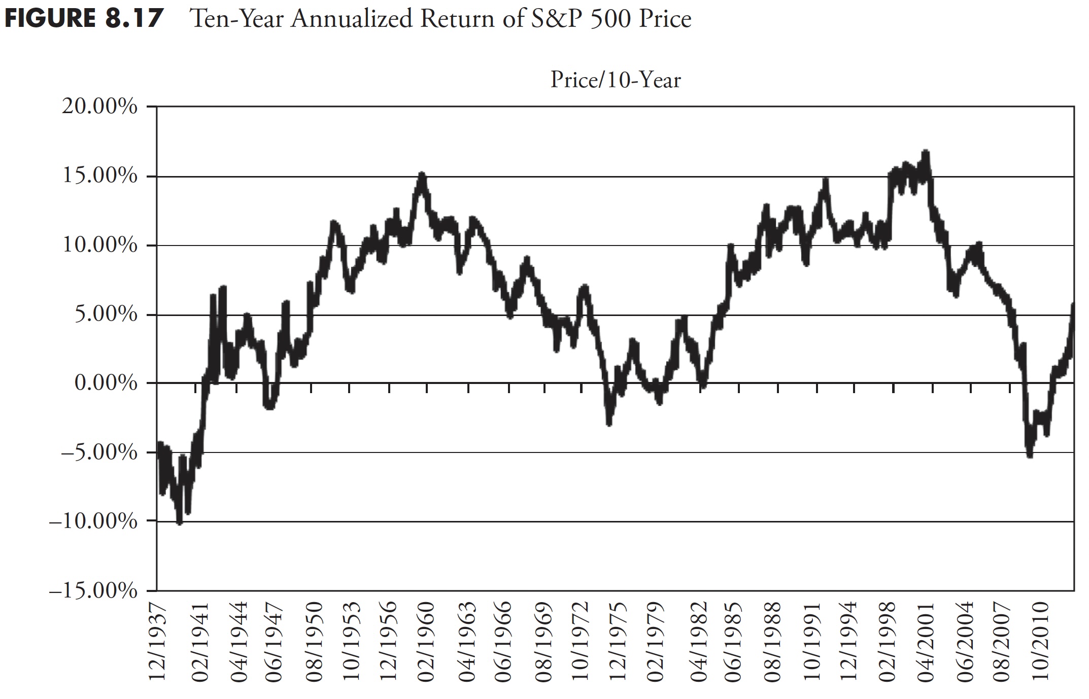
The ten-year return chart now clearly exhibits up-and-down tendencies within the knowledge (see Determine 8.17).
The 20-year rolling return chart (Determine 8.18) continues to scale back the short-term volatility within the chart, and the up-and-down tendencies change into clear.
Since I adamantly consider that almost all buyers have about 20 years to actually put cash away in a severe method for retirement, the next two charts present returns over 20 years for whole return (Determine 8.19) and inflation-adjusted whole return (Determine 8.20).
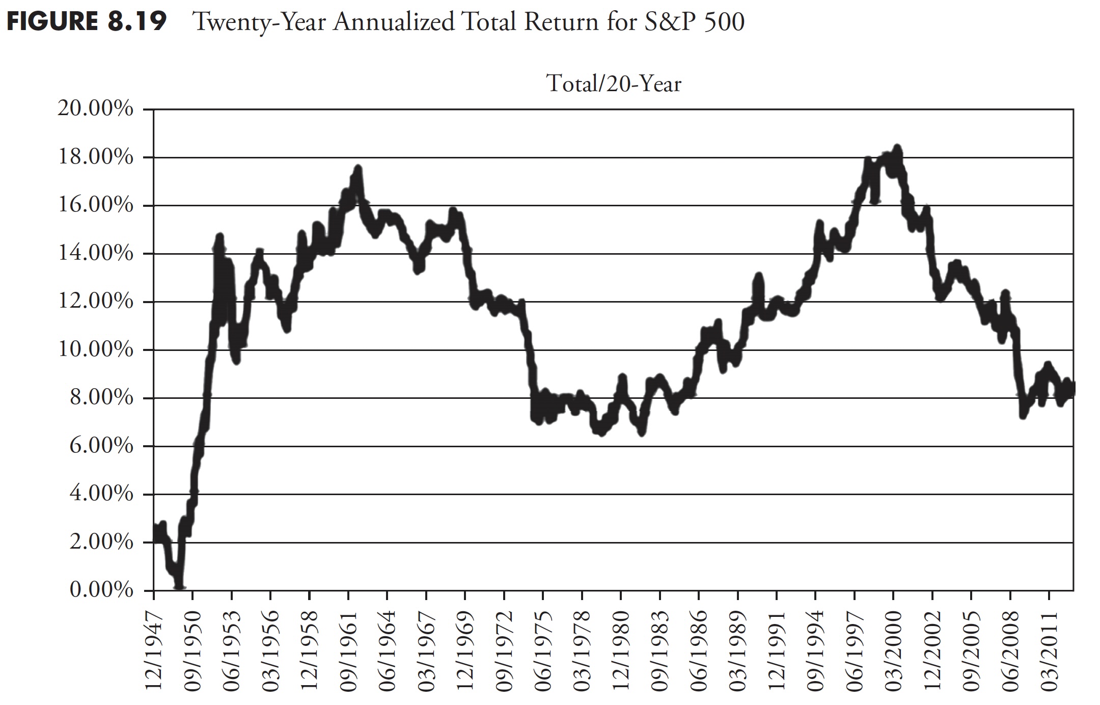
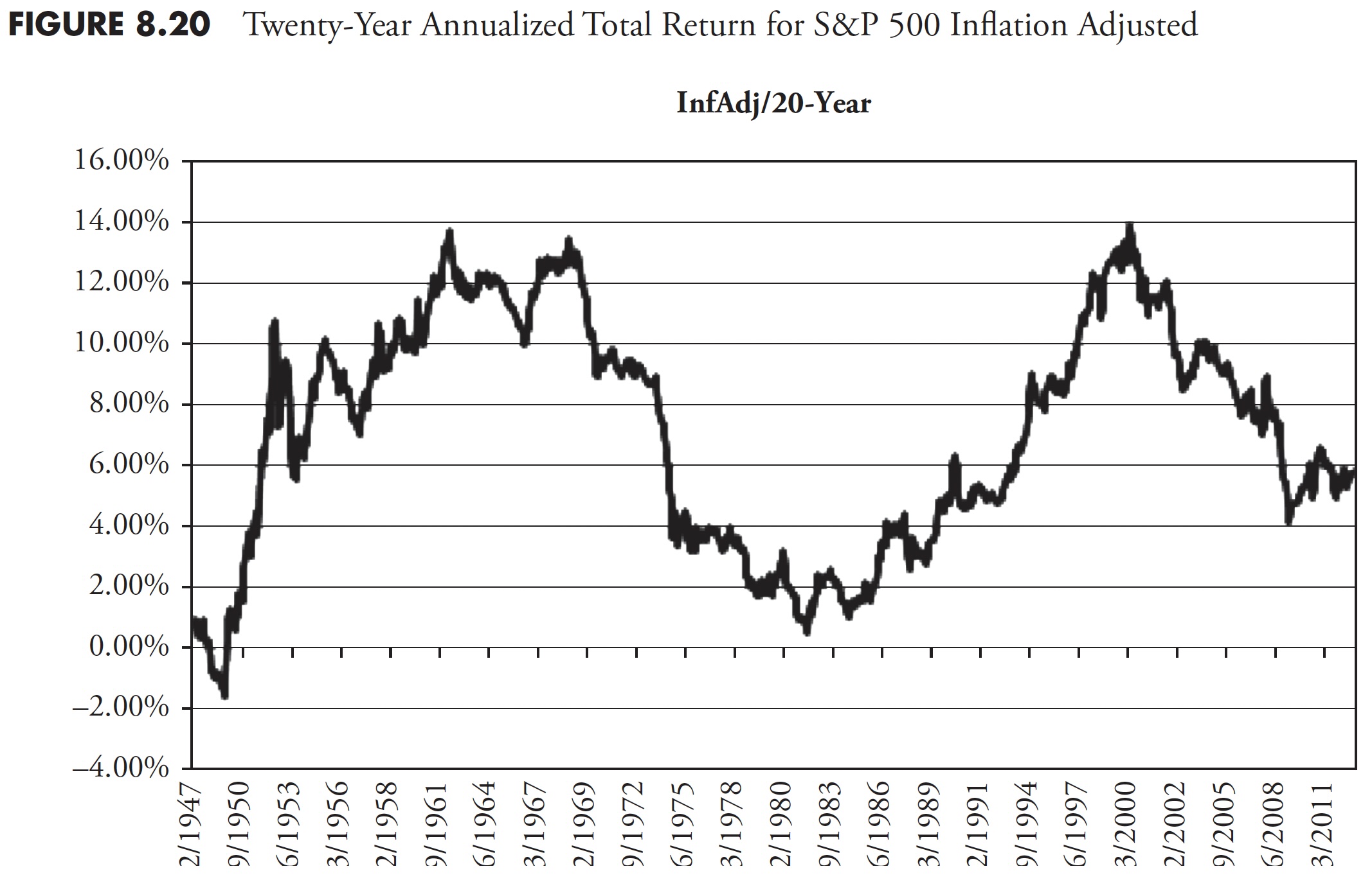
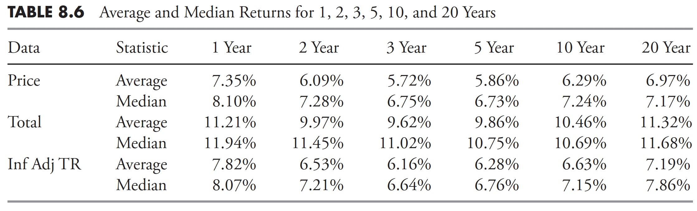
For many evaluation, the Worth chart is greater than satisfactory. On the planet of finance, there may be an virtually common demand for the Complete Return chart; nevertheless, I feel that if you’re going to insist on Complete Return, you need to then additionally insist on Inflation-Adjusted Complete Return. Utilizing the three previous 20-year charts and the averages proven, you’ll be able to see that the common for Worth is 6.97 %, Complete Return is 11.32 %, and Inflation-Adjusted Complete Return is 7.19 %. What this says is that the impact of together with dividends (Complete Return) and the impact of Inflation typically neutralize one another.
Desk 8.6 exhibits the annualized returns for the S&P 500 for value, whole return, and inflation-adjusted whole return for the next intervals: 1-year, 2-year, 3-year, 5-year, 10-year, and 20-year.
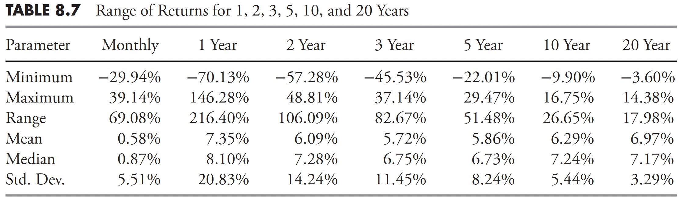
Desk 8.7 exhibits the minimal and most returns, together with the vary of returns, their imply, median, and variability about their imply (Customary Deviation).
Distribution of Returns
The vary of return knowledge could be very straightforward to calculate as a result of it’s merely the distinction between the biggest and the smallest values in an information set. Thus, vary, together with any outliers, is the precise unfold of knowledge. Vary equals the distinction between highest and lowest noticed values. Nevertheless, a substantial amount of data is ignored when computing the vary, as a result of solely the biggest and smallest knowledge values are thought of. The vary worth of an information set is drastically influenced by the presence of only one unusually giant or small worth (outlier). The drawback of utilizing vary is that it doesn’t measure the unfold of many of the values—it solely measures the unfold between highest and lowest values. Consequently, different measures are required with a view to give a greater image of the info unfold. The month-to-month returns for the S&P 500 start with December 1927, so, as of December 2012, there are 1,020 months (85 years) of knowledge.
Extra charts present the distribution of knowledge in varied methods utilizing the 20-year annualized returns of the S&P 500 inflation-adjusted whole return knowledge for rolling 20-year intervals. Twenty-year returns from the S&P 500 with 1,020 months of knowledge would yield 778 knowledge factors. Return distributions may be considered like this: Every bar represents the proportion of the returns that meet a proportion division of the info, mathematical division of the info, or statistical division of the info. The next are definitions of the assorted distribution strategies, as proven within the title of the next figures.
- Decile. Considered one of 10 teams containing an equal variety of the objects that make up a frequency distribution. The vary of returns is decided by the distinction between the minimal and most returns within the sequence, then divided by 10 to create 10 equal teams.
- Quartile. The calculation is much like decile (above), however with solely 4 groupings.
(Be aware: This use of decile and quartile doesn’t comply with the usual definition or calculation methodology typically utilized in statistics.)
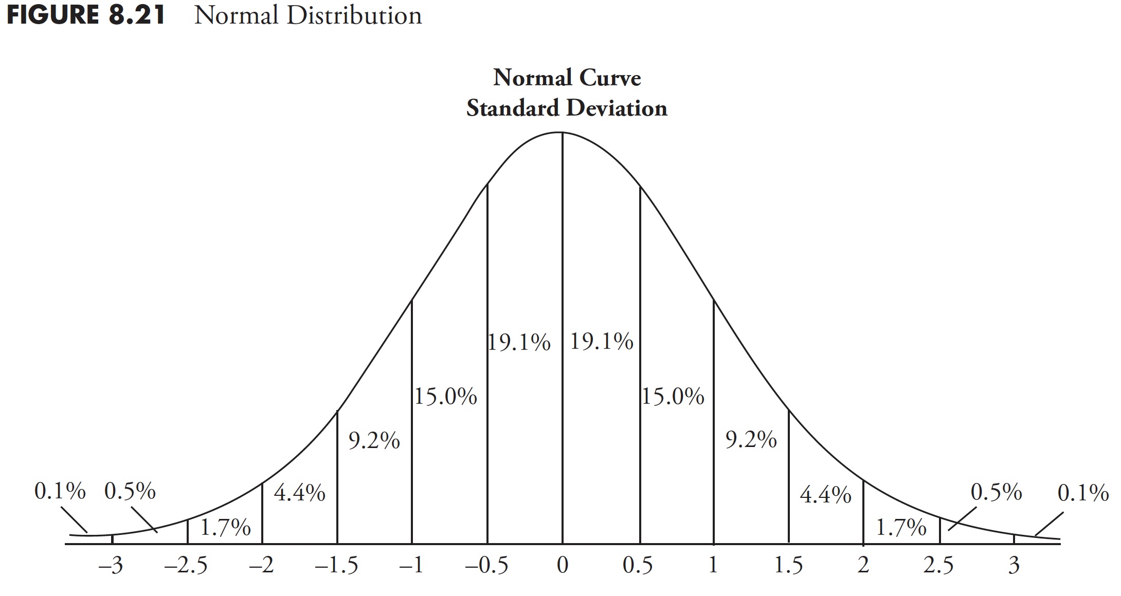
- Customary deviation. A statistical measure of the quantity by which a set of values differs from the arithmetical imply, equal to the sq. root of the imply of the variations’ squares. Determine 8.21 exhibits the proportion of the info that’s included in a normal deviation. You’ll be able to see that the imply is the height and that 68.2 % of the info is inside one normal deviation from the imply, and 95.4 % of the info is inside two normal deviations of the imply.
- Proportion. A proportion acknowledged by way of one-hundredths that’s calculated by multiplying a fraction by 100.
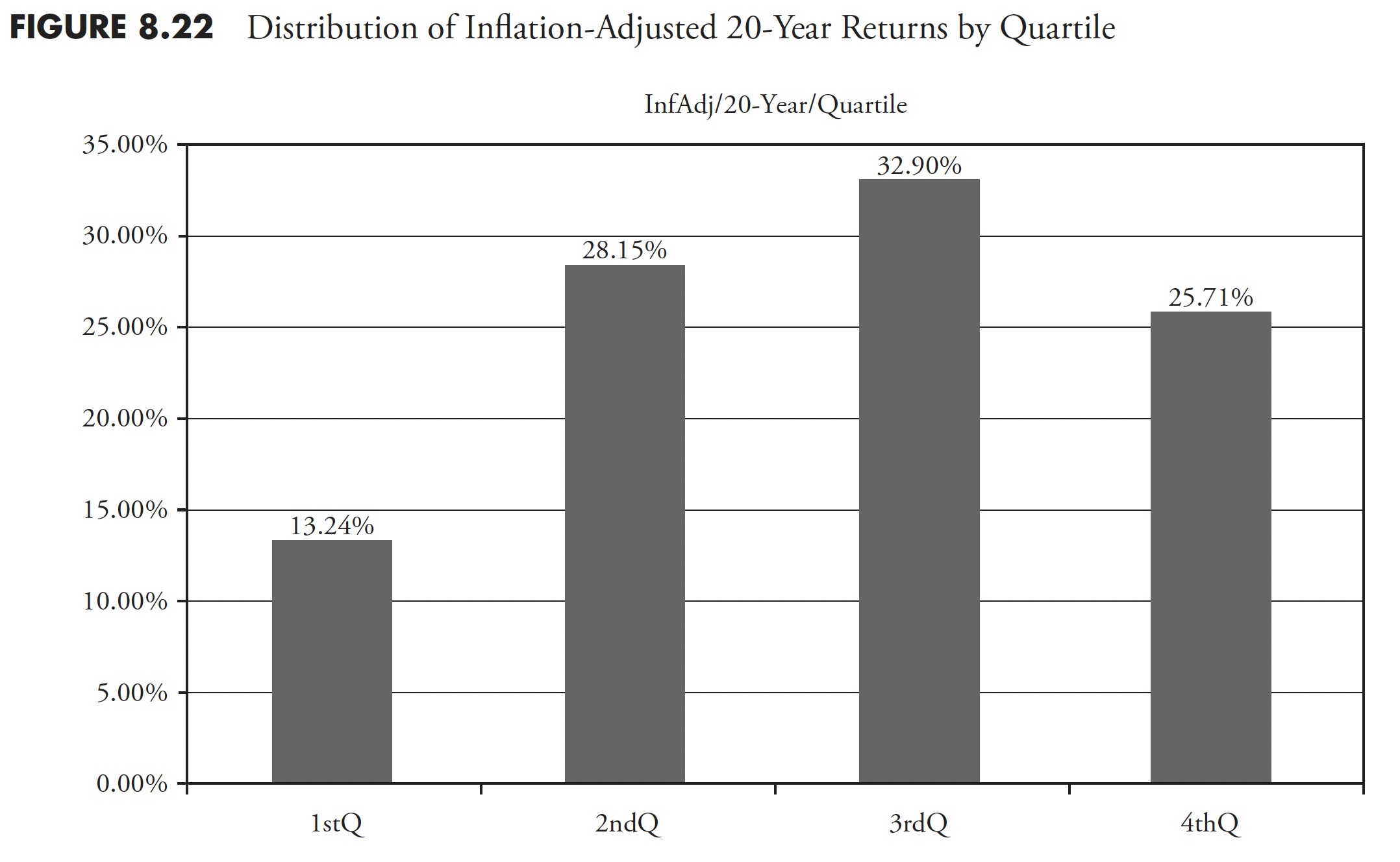
Determine 8.22 exhibits the 20-year rolling returns utilizing inflation-adjusted whole return knowledge distributed by quartiles. From the chart, you’ll be able to see that 13.24 % of the returns fall into the primary quartile, or lowest 25 %, of the info, 28.15 % within the second, 32.90 % within the third, and 25.71 % within the fourth quartile or highest 25 % of the info.
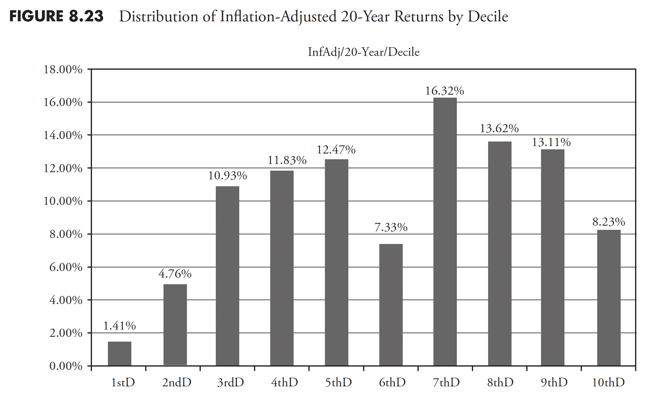
Determine 8.23 exhibits the identical knowledge, however in a decile distribution the place every bar represents 10 % of the variety of knowledge objects. For instance, 8.23 % of the info fell within the highest 10 % of the info.
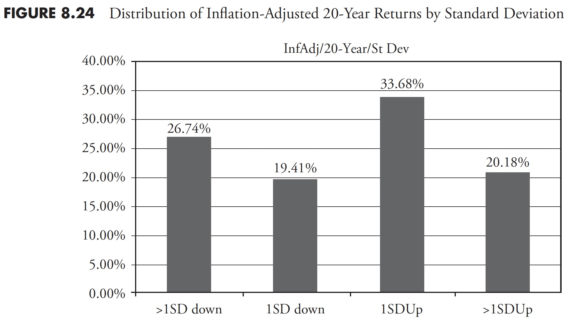
Determine 8.24 exhibits the distribution of the info based mostly on variance from the imply or normal deviation. You’ll be able to see that the 2 center bars every symbolize 34.1 % of the info (68.2 % whole) that’s one normal deviation from the imply. For example, 33.68 % of the 20-year rolling returns knowledge was inside one normal deviation above the imply of all the info. You may also surmise that the 2 bars on the precise symbolize 50 % of all the info and 53.86 % (33.68 + 20.18) of the returns. Oversimplifying this, one then is aware of that there have been extra returns better than the imply. Nevertheless, there may be an asymmetrical distribution between the returns which can be outdoors of 1 normal deviation from the imply, with the bigger proportion to the draw back.
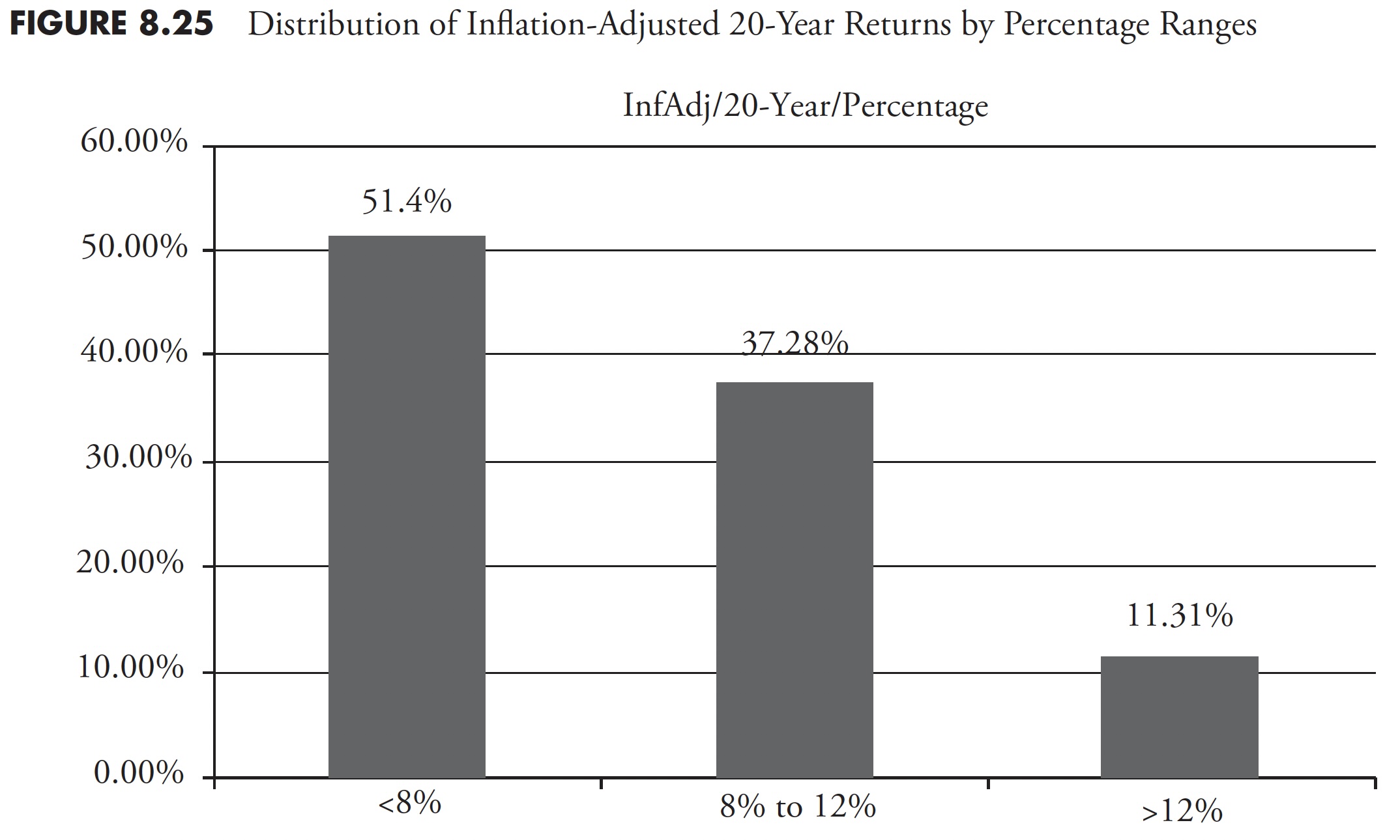
Determine 8.25 exhibits the 20-year rolling returns of the S&P 500 inflation-adjusted whole return inside proportion ranges. The bar on the left exhibits all of the returns of lower than 8 %, which accounted for greater than 50 % of all returns (51.41 %), whereas the bar on the precise exhibits returns of better than 12 %, accounted for under 11.31 % of all returns. The bar within the center is the vary of returns between 8 % and 12 %, which accounted for 37.28 % of all returns. Recall the dialogue in Chapter 4 on the deception of common, and as soon as once more the common 8 % to 12 % return is just not common.
When the market begins to say no considerably, it’s not the identical as when somebody yells “hearth” in a theater. In a theater, everyone seems to be working for the exits. In an enormous decline out there, you’ll be able to run for the exits, however first you must discover somebody to exchange you—it’s essential to discover a purchaser. Huge distinction! This chapter has tried to stay to what I consider are market information and important data you need to perceive in regard to how markets work and have labored up to now. If one doesn’t know market historical past, it could be very tough to maintain a deal with what the probabilities are sooner or later.
This concludes the primary part of this guide, the place I’ve tried to point out you the numerous in style beliefs in regards to the market which can be utilized by academia and Wall Road to assist promote their merchandise. Half I additionally wraps up with what I consider to be truisms in regards to the market. Half II has an introductory chapter on technical evaluation and is adopted by two chapters on intensive analysis into development dedication and threat/drawdowns.
Thanks for studying this far. I intend to publish one article on this sequence each week. Cannot wait? The guide is on the market right here.